

 Completed
Scattering parameter measurement device based on single-chip microcontroller
PRO Scattering parameter measurement device based on single-chip microcontroller
License
:GPL 3.0
Description
Chapter 1, System Scheme Design and Function Introduction
1.1 System scheme design
This design studies the scattering parameter measurement device. The device uses STM32H723ZGT6 as the control chip, and is connected to an external scattering Data Acquisition module and a display module. Among them, the scattering Data Acquisition module is the core part of the device, which can generate a sweep signal to excite the test system, separate the incident signal from the reflected signal through a directional bridge, mix the signal through a superheterodyne structure, and use an ADC chip to collect the signal. The display module supports measurement parameter switching, display mode switching, range selection and other functions through a self-designed UI interface. The interfaces between each module are introduced with "horns", connected through IDC cables, and easy to connect while preventing reverse connection. We use this device to measure the amplitude-frequency and phase-frequency characteristics of each frequency point of the test system, and then calculate the S parameters of the test system (including S11, S12, S21, S22), and then calculate the impedance continuity, reflection coefficient, electrical length and other related properties of the test system. The overall framework of the scattering parameter measurement device is shown in Figure 1.1.

Figure 1.1 Overall block diagram of scattering parameter measurement device
The scattering Data Acquisition module is responsible for implementing four key module functions: sweep signal source, directional bridge, mixer, and ADC synchronous signal acquisition. Among them, the signal source is used to excite the test system, the directional coupler is used to separate the S11 echo and inject excitation, the mixer is used for down-conversion, and the local oscillator is the down-converted signal source. After the test signal is down-converted, it is necessary to simultaneously mix and analyze the excitation signal generated by the signal source to achieve the solution of scattering parameters. Thanks to the high-performance digital circuit, all down-converted signals can be directly sent to the ADC for synchronous sampling after passing through an anti-aliasing filter, and finally digital signal processing.
1.2 Main technical features
1.2.1 use square wave signals as signal sources
The signal source is selected from the chip Si5351A, which is itself a clock generator that can be used to generate square wave clock signals with frequencies of 8kHz-160MHz. Compared with the sinusoidal signal of the same frequency, the odd harmonics (third harmonic, fifth harmonic, etc.) of the square wave can also be used as excitation signals. Therefore, the 160MHz square wave signal can not only be used as a test signal of 160MHz, but also as a test signal of 480MHz (third harmonic) or 800MHz (fifth harmonic). By configuring the registers corresponding to the frequency doubling coefficient and frequency dividing coefficient of the clock chip Si5351 through the program, a sweep signal of 8kHz~ 800MHz can be obtained.
1.2.2 superheterodyne structure
The excitation signal (i.e. incident signal) generated by the chip Si5351A, the reflection signal of the equipment under test, and the output signal of the equipment under test will all be downconverted to 5kHz through the mixer chip SA612AD with another local oscillator signal generated by the chip Si5351A. The downconverted output signal can be passed through a low-pass filter and then passed into the ADC chip for sampling. In order to ensure that all signals can be downconverted to 5kHz, it is necessary to achieve fS - fL = 5kHz, where fS is the frequency of the excitation signal generated by the chip Si5351A and fL is the frequency of another local oscillator signal generated by the clock chip Si5351. The superheterodyne receiver structure is shown in Figure 1.2.
![@L{XYST`ZHM6)]9V)VXE%ZT](http://image.lceda.cn/pullimage/SBK4Dgj5yi0QGRI6e54g0jLjfXwnjVPSaKzUSzIg.png)
1.3 Performance indicators
|
Basic parameter |
Performance index |
|
Scattering parameters measure frequency range |
50kHz - 300MHz |
|
frequency resolution |
1kHz |
|
Amplitude-frequency response measurement error |
Less than 5% |
|
Phase frequency response measurement error |
Less than 5% |
|
Coaxial cable length measurement range |
0.1m - 20m |
|
Coaxial cable length measurement error |
Less than 1% |
|
Measured response time |
Less than 3S |
|
Whether there is a self-correcting function |
yes |
Chapter 2, software design and algorithm implementation of scattering parameter measurement device
2.1 Program flowchart
2.1.1 main program flowchart
After the device is powered on and started, each functional module will be initialized. After the initialization is completed, function selection can be performed through the serial port screen. Port calibration is preferred to eliminate system errors in the test system. The second step is to set the test frequency range: configure the scattering parameter measurement device to cover the required frequency range. The third step is to set the scattering parameters to be measured, such as S11, S21, etc. The fourth step is to measure: after starting the measurement, the scattering parameter measurement device will send a test sweep signal to the device under test, and measure the output signal at the corresponding port to calculate the corresponding S parameters based on the amplitude, phase, and other information of the output signal and the test signal. The fourth step is to select the data display method and content: the coordinate axis is linear and logarithmic, and the measurement content has amplitude and phase options. The final step is to record and analyze the results: you can choose to record the measurement results in flash for subsequent storage, reading, and analysis. The specific flowchart of the main program is shown in Figure 2.1.

Figure 2.1 Flowchart of the main program of the scattering parameter measurement device
2.1.2 Scattering Parameter Measurement Flowchart
The single-chip microcomputer first controls the clock chip Si5351 to generate a linear sweep signal based on the selected test frequency range, then controls the AD7606 to sample the input and output signals. After the sampling is completed, the sampling results are analyzed, and the set S parameters are calculated based on the calibration data, and finally displayed on the serial screen. The specific flowchart for measuring and calculating scattering parameters is shown in Figure 2.2.

2.2 Single-port reflection coefficient measurement and system error correction
Single-port system error calibration includes OSM (open/short/match, also known as OSL - open/short/load). OSL calibration belongs to full single-port calibration, which can correct the error terms involved in comprehensive single-port testing and effectively improve the accuracy of testing single-port devices.
The basic process of reflection testing: the excitation source provides a signal, which is mostly output to the DUT through the vector network port after passing through the coupler; the signal reflected by the DUT passes through the coupling path of the coupler to the measurement receiver Meas. Receiver. Since the vector network port also has reflection, assuming the reflection coefficient is S, there will be multiple reflections between the vector network port and the DUT port, and the amount of multiple reflections will also enter the Meas. Receiver through the coupling path. In addition, because the coupler is not ideal, its isolation degree is also limited, which leads to a part of the excitation signal being directly fed into the Meas. Receiver through the isolation channel of the coupler. That is to say, Meas. The signal received by the receiver actually consists of three parts: the signal directly reflected by the DUT, the multiple reflected signals at the test reference surface, and the signal directly leaked through the coupler isolation channel. The entire process of the signal from source transmission to receiver reception is shown in Figure 2.3.

The coupler itself has 4 ports, but considering that only some parameters of the coupler are involved in this model, it is equivalent to a 3-port device here, with ports being port1, port2, and port3. S21 refers to the through transmission coefficient of the coupler, the transmission coefficient of the leakage channel, and the transmission coefficient of the coupling channel. For simplicity, the signal flow diagram in Figure 4.3 can be drawn first, as shown in Figure 2.4, where the true reflection coefficient of the DUT is shown.

The expression of b3 can be directly obtained from the signal flow graph.
The measurement values of the reflection coefficient obtained by simplification are as follows:
From the above equation, it can be seen that there are four error terms in the measurement of reflection coefficient:,,, S. Generally referred to as (), it is called reflection tracking R (Reflective Tracking), which is called directivity, abbreviated as D (Directivity), and S is called source matching.
After simplification, there are actually three error terms, R, D, and S, in single-port testing. During calibration, three standard parts, Open, Short, and Match, are used respectively, and each standard part obtains an equation.
Among them, the reflection coefficients measured when the port is open-circuited, short-circuited, or matched can be solved by solving the equations to obtain the unique solutions of three error terms.
The true reflection coefficient can be inverted by using three error terms R, D, and S.
Where M is the measured reflection coefficient, which is the true reflection coefficient after correction.
Chapter 3, Device Test Results
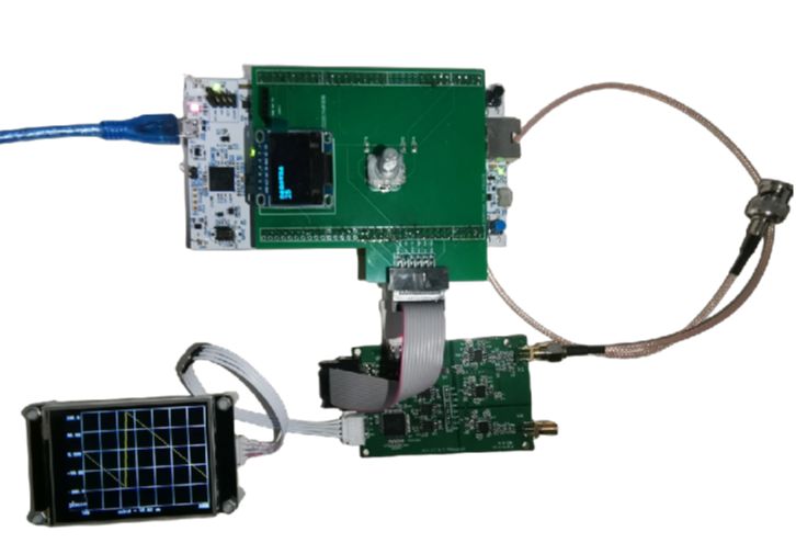
3.1 Device physical diagram

The scattering Data Acquisition module transmits a swept signal to the coaxial cable through a swept signal source. The directional bridge separates the incident signal and the reflected signal. The two signals are down-converted by the mixer and synchronously sampled through the ADC. The main control STM32H7 reads the sampling results of the two signals and performs spectral analysis through DFT. The amplitude-frequency characteristics and phase-frequency characteristics of the two signals are compared to obtain the amplitude-frequency characteristics and phase-frequency characteristics of each frequency point.
The main control STM32H7 sends the test results (including amplitude response and phase response) of each test frequency point to the computer for display through the serial port, as shown in Figure 3.2.

The main control STM32H7 calculates the length of the coaxial cable based on the propagation speed of electromagnetic waves in the coaxial cable and the phase difference between the reflected signal and the incident signal. Finally, the amplitude-frequency curve, phase-frequency curve, and coaxial cable length are displayed on the serial port screen. The left side of Figure 3.3 shows the amplitude-frequency response curve, and the right side of Figure 3.3 shows the phase-frequency response curve. The two curves can be switched and viewed by pressing buttons on the serial port screen.

Designed by textm (from OSHWHub)
Design Drawing
 Empty
Empty
Comment